
Digital Transformation, zBlog
Exploratory Data Analysis (EDA): Types, Tools, Process
Team Trantor | Updated: June 22, 2026

If you searched for “EDA full form” or “what is EDA,” here is the direct answer: EDA stands for Exploratory Data Analysis. It is the process of investigating a dataset — using statistics and visualizations — to understand its structure, spot patterns, and catch problems before you build any model on top of it.
That one-line definition is the easy part. The harder and more valuable question is what exploratory data analysis actually involves in practice, why it determines whether an entire analytics or machine learning project succeeds, and how data teams at real companies use it day to day. That is what this guide covers — in full, with the actual Python code, the real 7-step process used in enterprise projects, and the tools that data scientists rely on in 2026.
Data scientists spend roughly 80% of their project time on data cleaning and exploration before any model gets built. That exploration phase — exploratory data analysis — determines whether a project succeeds or stalls in a swamp of bad assumptions and overlooked patterns. With datasets in 2026 expanding rapidly from IoT sensors, customer interaction logs, and multimodal AI sources, EDA is not an optional preliminary step. It is the foundation that everything else stands on.
We have refined the techniques in this guide through real EDA engagements across finance, healthcare, and retail at Trantor. One pattern shows up consistently: teams that rush through or skip EDA discover the consequences of that decision in production — not in development. The cost of finding a data quality problem after a model is deployed is many times higher than catching it during exploration.
What Is Exploratory Data Analysis? The Complete Definition
Exploratory Data Analysis (EDA) is the process of investigating a dataset to summarize its main characteristics, often using visual methods, before applying formal statistical modeling or machine learning. EDA helps you understand data structure, detect anomalies, test assumptions, and discover patterns — all before you commit to a modeling approach.
Think of EDA as detective work. Instead of jumping straight to conclusions or building a model on data you have not actually looked at, you methodically investigate what the data is actually telling you. The term was popularized by statistician John Tukey in his 1977 book “Exploratory Data Analysis,” and the core philosophy has not changed in nearly 50 years: look at the data first, form hypotheses from what you see, and only then move to formal testing or modeling.
EDA Full Form and Common Variations
The full form of EDA is Exploratory Data Analysis. You will also see it referred to as “exploratory analysis,” “data exploration,” or simply “data profiling” — these terms largely overlap, though EDA is the most precise and widely used term in both academic and enterprise data science contexts.
In Machine Learning: EDA full form in ML is identical — Exploratory Data Analysis. In an ML context, EDA specifically focuses on understanding features before model training: identifying which variables correlate with the target, detecting multicollinearity, and spotting class imbalance in classification problems.
In Data Science: EDA in data science is the broader discipline — it is the second formal stage of the data science lifecycle, sitting between data collection/cleaning and formal statistical or predictive modeling.
KEY DISTINCTION:
EDA is not the same as descriptive statistics, though people often conflate the two. Descriptive statistics summarize what you already expect to find (mean, median, standard deviation). EDA is specifically oriented toward finding what you did NOT expect — the surprises, anomalies, and hidden relationships that a simple summary table would never reveal.
Why Exploratory Data Analysis Matters More Than Ever in 2026
Modern datasets are not just bigger than they were five years ago — they are messier. Structured CRM data mixes with unstructured social sentiment, time-series sensor readings, and vector embeddings from foundation models. Without rigorous EDA, organizations risk building models on skewed distributions, missing critical outliers that signal fraud or equipment failure, and wasting weeks engineering features that turn out not to correlate with the outcomes they care about.
Here is a real, concrete example of what EDA catches. A Trantor retail client ran exploratory analysis on their customer returns data and discovered that 15% of their “high-value” customers — segmented that way purely on transaction volume — were actually serial returns abusers gaming the loyalty program. That single insight, surfaced through EDA pattern detection rather than any predictive model, saved the client $2.7 million annually in fraudulent refunds. No machine learning model would have caught this on its own; it took a human looking carefully at distributions and groupings to notice the pattern.
EDA vs. Descriptive Statistics vs. Inferential Analysis
These three terms get confused constantly. Here is the clear distinction, visualized.

EDA asks “what is going on in this data that I do not yet understand?” Descriptive statistics asks “how do I summarize what I already know is there?” Inferential analysis asks “can I generalize this pattern to the broader population with statistical confidence?” All three matter. But EDA always comes first, because the hypotheses that descriptive statistics and inferential tests evaluate should come from genuine exploration — not assumptions made before looking at the data.
The Complete EDA Process: A 7-Step Framework
Effective exploratory data analysis follows a structured yet iterative workflow. Here is the 7-step process we have battle-tested across enterprise projects at Trantor — refined through real engagements, not just textbook theory.

Step 1 — Define Business Objectives and Data Questions
Start with why. What business problem does this analysis solve? Frame 3-5 specific questions before touching the data: “Which customer segments drive 80% of churn?” “What sensor readings predict equipment failure 48 hours early?” “Do marketing channels correlate with lifetime value after 90 days?”
Pro tip: Document your assumptions upfront. A statement like “we assume recent data reflects current behavior” becomes directly testable once you start exploring — and you will frequently find that assumption was wrong.
Step 2 — Data Collection and Initial Quality Check
Gather data from every relevant source — CRM systems like Salesforce or HubSpot for customer demographics and transactions, web analytics for behavior and acquisition source, IoT or ERP systems for operational metrics, social APIs for sentiment and engagement.
import pandas as pd

df = pd.read_csv('customer_data.csv')

print(f"Shape: {df.shape}")
print(f"Missing values:\n{df.isnull().sum()}")
print(f"Data types:\n{df.dtypes}")
print(f"Duplicates: {df.duplicated().sum()}")
Step 3 — Univariate Analysis: Understanding Individual Variables
Analyze each feature independently to establish baselines before looking at relationships between variables.
import matplotlib.pyplot as plt
import seaborn as sns

# Numerical features — histogram + boxplot
df['age'].hist(bins=30)
plt.title('Customer Age Distribution')
sns.boxplot(y=df['age'])

# Categorical features
df['region'].value_counts().plot(kind='bar')
plt.title('Customer Distribution by Region')
Key metrics to compute: Mean, median, mode, standard deviation, interquartile range (IQR), skewness, kurtosis, min/max, and key percentiles (5th, 95th).
Step 4 — Bivariate and Multivariate Analysis: Finding Relationships
This step reveals correlations and interactions between variables — often the most valuable phase of EDA, because relationships between features are rarely obvious from looking at any single column alone.
# Correlation heatmap
plt.figure(figsize=(12,8))
sns.heatmap(df.corr(), annot=True, cmap='coolwarm')

# Scatter plots for key pairs
sns.scatterplot(x='tenure', y='monthly_charges', hue='churn', data=df)

# Pair plots for multiple relationships
sns.pairplot(df[['age', 'tenure', 'charges', 'churn']], hue='churn')
2026 ADDITION:
For projects involving AI embeddings (common in 2026 RAG and recommendation systems), vector similarity analysis is now a standard EDA technique: from sklearn.metrics.pairwise import cosine_similarity applied to embedding columns reveals semantic clustering that traditional correlation analysis cannot capture.
Step 5 — Outlier Detection and Treatment
Outliers are not always errors — they often contain the most important signal in the dataset.
# IQR method
Q1 = df['charges'].quantile(0.25)
Q3 = df['charges'].quantile(0.75)
IQR = Q3 - Q1
outliers = df[(df['charges'] < Q1 - 1.5*IQR) | (df['charges'] > Q3 + 1.5*IQR)]

# Isolation Forest (multivariate outlier detection)
from sklearn.ensemble import IsolationForest
iso = IsolationForest(contamination=0.05)
df['outlier'] = iso.fit_predict(df[num_cols])
Business judgment matters here: flag a $50,000+ single transaction for fraud review — do not simply delete it as “bad data.” The outlier itself may be the finding.
Step 6 — Missing Data Diagnosis and Imputation Strategy
# Missing data heatmap
sns.heatmap(df.isnull(), cbar=True, yticklabels=False)

# Missing by group — reveals if missingness is random or systematic
df.groupby('region')['income'].apply(lambda x: x.isnull().sum())
Imputation strategies, chosen per context: mean or median for numerical features, mode for categorical features, KNN or time-series forward-fill for advanced cases, and increasingly in 2026, LLM-generated synthetic data for complex missingness patterns where simple imputation would distort the underlying distribution.
Step 7 — Feature Engineering and Transformation Insights
EDA reveals transformation opportunities that would not be obvious without first exploring the data.
# From EDA insights: create derived features
df['charge_per_month_tenure'] = df['charges'] / df['tenure']
df['is_high_value'] = (df['charges'] > df['charges'].quantile(0.9)) & (df['tenure'] > 24)

# Log transformation for skewed data
import numpy as np
df['log_charges'] = np.log1p(df['charges'])

# Binning for interpretability
df['age_group'] = pd.cut(df['age'], bins=[0, 25, 40, 60, 100],
                          labels=['Young', 'Adult', 'Middle', 'Senior'])
Types of Exploratory Data Analysis — Univariate, Bivariate, Multivariate, Graphical, and Non-Graphical
A common way to categorize EDA is along two dimensions: how many variables you are examining at once, and whether you are using visual or purely numerical methods.
Univariate Analysis: Examines one variable at a time. Includes both graphical methods (histograms, box plots) and non-graphical methods (computing mean, median, mode, and standard deviation for that single variable).
Bivariate Analysis: Examines the relationship between exactly two variables. Scatter plots, correlation coefficients, and cross-tabulations fall into this category — this is how you discover, for example, that customer tenure and monthly charges interact differently for customers who eventually churn versus those who do not.
Multivariate Analysis: Examines relationships among three or more variables simultaneously. Correlation heatmaps, pair plots, and dimensionality reduction techniques like PCA are the standard tools here.
Graphical EDA: Any technique that relies on visualization — histograms, box plots, scatter plots, heatmaps. Graphical methods are typically faster for humans to interpret and better for communicating findings to non-technical stakeholders.
Non-Graphical EDA: Purely numerical summary techniques — computing means, variances, correlation coefficients, and quantiles without visualization. Often used as a first quick pass before investing time in plots, or in automated pipelines where visual inspection is not practical.
Essential EDA Tools and Libraries for 2026
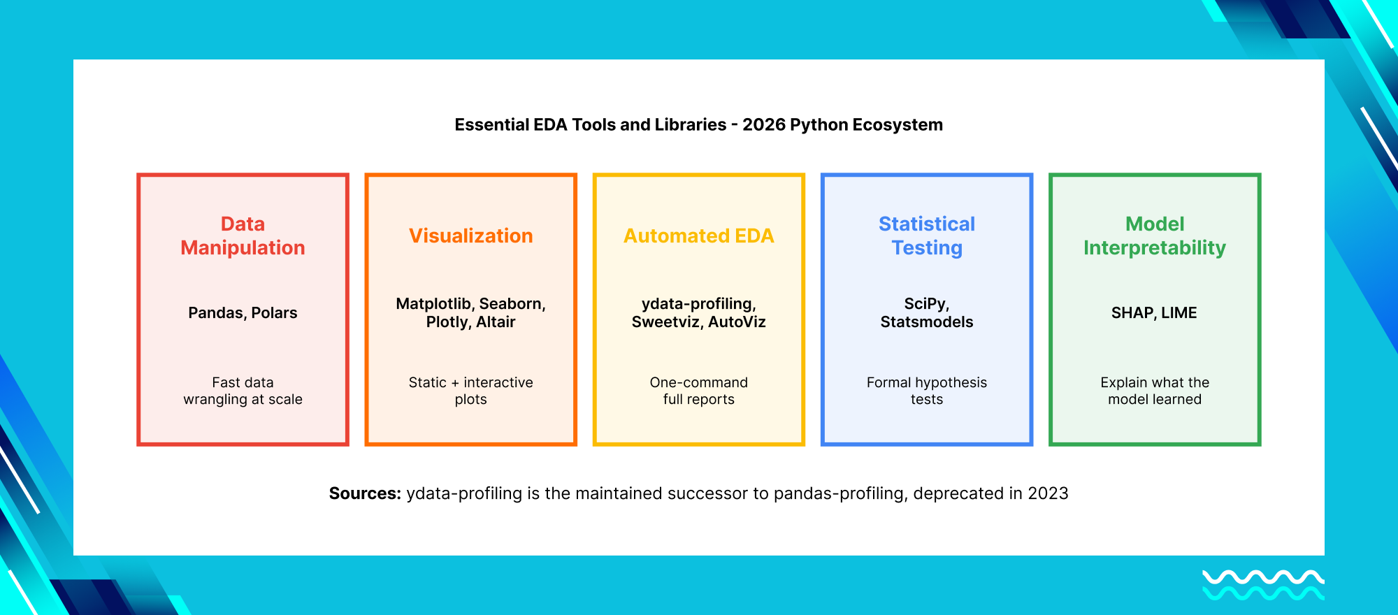
The 2026 Power Combo — Automated EDA in 5 Lines
import pandas as pd
import ydata_profiling as ppf  # Successor to pandas-profiling

# Automated EDA report
profile = ppf.ProfileReport(df, title="Customer EDA Report")
profile.to_file("eda_report.html")
R Ecosystem (Statistical Teams)
library(tidyverse)
library(DataExplorer)
library(visdat)

# One-liner EDA
DataExplorer::plot_intro(df)
No-Code/Low-Code Tools: Tableau Prep handles visual data prep and EDA without writing code. Power BI Dataflows integrate naturally with the Microsoft enterprise stack. Hex and Deepnote provide collaborative notebooks with built-in EDA capabilities for teams that want shareable, interactive analysis.
EDA Visualization Best Practices — What to Use and When
Must-Have EDA Visualization by Data Types
| Data Type | Recommended Viz | Python Code |
|---|---|---|
| Numerical | Histogram + Box Plot | sns.histplot() + sns.boxplot() |
| Categorical | Count Plot + Treemap | sns.countplot() + squarify |
| Time-Series | Line + Seasonal Decomp | px.line() + seasonal_decompose() |
| Bivariate | Scatter + Correlation Heatmap | sns.scatterplot() + sns.heatmap() |
| Geospatial | Choropleth + Heatmap | geopandas + folium |
Start simple (histograms) before complex (heatmaps) — sequence matters for stakeholder communication
| Numerical | |
|---|---|
| Recommended Viz | Histogram + Box Plot |
| Python Code | sns.histplot() + sns.boxplot() |
| Categorical | |
|---|---|
| Recommended Viz | Count Plot + Treemap |
| Python Code | sns.countplot() + squarify |
| Time-Series | |
|---|---|
| Recommended Viz | Line + Seasonal Decomp |
| Python Code | px.line() + seasonal_decompose() |
| Bivariate | |
|---|---|
| Recommended Viz | Scatter + Correlation Heatmap |
| Python Code | sns.scatterplot() + sns.heatmap() |
| Geospatial | |
|---|---|
| Recommended Viz | Choropleth + Heatmap |
| Python Code | geopandas + folium |
Start simple (histograms) before complex (heatmaps) — sequence matters for stakeholder communication
Principles that convert insights into action: Start simple — histograms before heatmaps. Use color purposefully — sequential color scales for magnitude, diverging scales for deviation from a midpoint, qualitative palettes for categories. Prefer faceting over overlaying when comparing groups (sns.FacetGrid()). Choose interactive over static visualizations for stakeholder demos (Plotly Dash). And always annotate — a chart without an explanation of why the pattern matters is just decoration.
Common EDA Pitfalls and How to Avoid Them

1. Confirmation Bias: Seeing patterns that confirm what you already expected to find, while overlooking patterns that contradict your assumptions. Fix: document your null hypotheses before exploring, and where possible run a first pass of analysis blind to the outcome variable.
2. Over-Cleaning: Removing “messy” data points that actually contain real signal — particularly dangerous with outliers and rare-category values. Fix: version your datasets at each cleaning stage and test model performance with and without aggressive cleaning to see what is actually being lost.
3. P-Hacking: Testing so many relationships during exploration that some appear statistically significant purely by chance. Fix: pre-register your key hypotheses before the exploration phase, and apply corrections like the Bonferroni adjustment when testing multiple comparisons.
4. Ignoring the Data Generation Process: Treating survey data with the same statistical assumptions as transaction data, when the two have fundamentally different collection biases and noise structures. Fix: map your data back to the actual business process that generated it during Step 1, before any analysis begins.
5. Treating All Outliers as Errors: Automatically removing extreme values without investigating whether they represent fraud, equipment failure, or another genuinely important signal. Fix: always investigate before you delete — the $2.7 million fraud detection example earlier in this guide came from outliers that a less careful analyst would have simply discarded.
Frequently Asked Questions About Exploratory Data Analysis (EDA)
Conclusion: EDA Is the Foundation, Not a Formality
Exploratory Data Analysis is not a box to check before the “real” work of modeling begins. It is the work that determines whether everything built afterward is trustworthy. The 80% of project time that data scientists spend on cleaning and exploring data is not waste — it is the investment that prevents the much larger waste of building, deploying, and eventually discarding a model trained on data nobody actually understood.
Whether you are working through your first customer churn analysis or running EDA across a multimodal dataset combining text, sensor readings, and embeddings, the same discipline applies: look at the data before you assume anything about it. Follow a structured process. Treat outliers and missing data as information, not noise to be discarded. And always tie your exploration back to the specific business question you are trying to answer.
At Trantor (trantorinc.com), we help U.S. organizations across finance, healthcare, and retail turn raw, messy data into production-grade insight — starting with the exploratory analysis that most teams rush past. Our data science and analytics teams have run EDA at enterprise scale, catching the kind of patterns that saved one client $2.7 million annually in fraud losses alone. Whether you need a one-time data audit before a major ML initiative, an ongoing analytics practice, or a team to build the dashboards and pipelines that make exploratory analysis a continuous capability rather than a one-time event — that is the work we are built for.